Pre-Delivery Walkthrough: SCHISM + SFINCS over the Mendocino Coast¶

End-to-end demo of the coastal_calibration library and nwm_coastal QGIS plugin against a single Pacific coastal subdomain (Mendocino / Point Arena, CA). The walkthrough covers:

1. Draw the SCHISM subset polygon in QGIS with the plugin's Draw Polygon tool, then save it as extract_poly.geojson.
2. Extract a sub-mesh from the full Pacific SCHISM domain using that polygon, then run the SCHISM pipeline on the subdomain.
3. Derive the SFINCS inputs in QGIS: turn the extracted SCHISM mesh boundary into an SFINCS AOI polygon and pick the NWM flowlines that enter the domain.
4. Build & run the SFINCS model on the same boundary.
5. Compare modeled water levels against a NOAA CO-OPS tide gauge in a single 3-line plot (Observed, SCHISM, SFINCS).
6. Animate SCHISM and SFINCS water-level fields side-by-side with a shared colorbar.

Both simulations are 50 hours long and run locally in roughly 4 minutes each on this machine; no HPC is required.

0. Setup¶

The walkthrough runs out of docs/examples/walkthrough/. That directory is committed with the four input GeoJSONs the demo needs (extract_poly.geojson, aoi.geojson, refine_poly.geojson, discharge_nwm.geojson). Sections 1 and 3 below document the QGIS steps that produce these files. The full Pacific SCHISM mesh and the WRF geogrid are not redistributable, so they live as symlinks (model, geo_em_CONUS.nc) pointing at the proprietary data drive (see docs/examples/README.md for how to set them up).

In [1]:

from __future__ import annotations

import os
from pathlib import Path

notebook_dir = Path.cwd()  # assumes run from docs/examples/notebooks/
walkthrough_dir = (notebook_dir.parent / "walkthrough").resolve()
os.chdir(walkthrough_dir)

required = (
    "model",  # symlink to proprietary Pacific SCHISM mesh
    "geo_em_CONUS.nc",  # symlink to proprietary WRF geogrid
    "extract_poly.geojson",  # SCHISM subset polygon
    "aoi.geojson",  # SFINCS AOI (mesh boundary unioned with NHF divides)
    "refine_poly.geojson",  # SFINCS quadtree refinement zone
    "discharge_nwm.geojson",  # NWM flowlines crossing the AOI
)
missing = [n for n in required if not (walkthrough_dir / n).exists()]
if missing:
    raise FileNotFoundError(
        f"Required walkthrough inputs missing: {missing}. "
        "See docs/examples/README.md for setup instructions."
    )

print(f"Working directory: {walkthrough_dir}")
print("Inputs:")
for name in required:
    p = walkthrough_dir / name
    if p.is_symlink():
        kind = f"symlink -> {p.resolve()}"
    elif p.is_file():
        kind = f"file ({p.stat().st_size / 1e3:.1f} KB)"
    else:
        kind = "missing"
    print(f"  {name:<28s} {kind}")

from __future__ import annotations import os from pathlib import Path notebook_dir = Path.cwd() # assumes run from docs/examples/notebooks/ walkthrough_dir = (notebook_dir.parent / "walkthrough").resolve() os.chdir(walkthrough_dir) required = ( "model", # symlink to proprietary Pacific SCHISM mesh "geo_em_CONUS.nc", # symlink to proprietary WRF geogrid "extract_poly.geojson", # SCHISM subset polygon "aoi.geojson", # SFINCS AOI (mesh boundary unioned with NHF divides) "refine_poly.geojson", # SFINCS quadtree refinement zone "discharge_nwm.geojson", # NWM flowlines crossing the AOI ) missing = [n for n in required if not (walkthrough_dir / n).exists()] if missing: raise FileNotFoundError( f"Required walkthrough inputs missing: {missing}. " "See docs/examples/README.md for setup instructions." ) print(f"Working directory: {walkthrough_dir}") print("Inputs:") for name in required: p = walkthrough_dir / name if p.is_symlink(): kind = f"symlink -> {p.resolve()}" elif p.is_file(): kind = f"file ({p.stat().st_size / 1e3:.1f} KB)" else: kind = "missing" print(f" {name:<28s} {kind}")

Working directory: docs/examples/walkthrough
Inputs:
  model                        symlink -> /Volumes/data/schism_models/pacific
  geo_em_CONUS.nc              symlink -> /Volumes/data/schism_models/geo_em_CONUS.nc
  extract_poly.geojson         file (1.3 KB)
  aoi.geojson                  file (131.6 KB)
  refine_poly.geojson          file (223.9 KB)
  discharge_nwm.geojson        file (58.4 KB)

1. QGIS plugin: draw the SCHISM subset polygon¶

The walkthrough starts in QGIS, where the nwm_coastal plugin turns the full Pacific SCHISM mesh into a coastal subset polygon. The output of this section is extract_poly.geojson, the first input that the SCHISM pipeline in Section 2 consumes.

The walkthrough has this file pre-staged in docs/examples/walkthrough/extract_poly.geojson, so the SCHISM section below runs without QGIS. The steps below document how it was produced.

Step 1: Install the plugin and view the toolbar¶

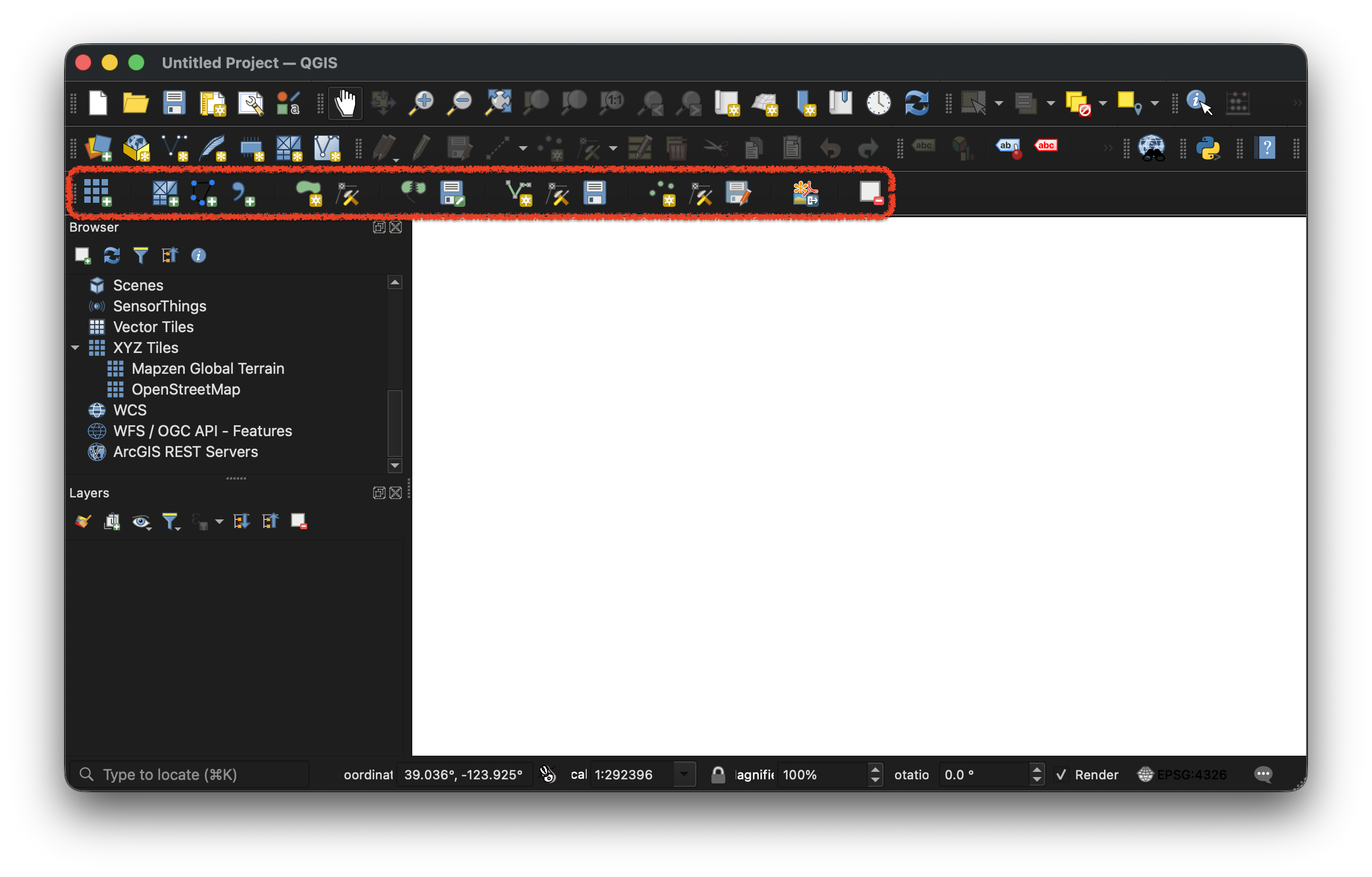
After installing the plugin, restart QGIS. The nwm_coastal toolbar appears as the highlighted row of icons below, with one icon per pipeline step in left-to-right order.

Step 2: Add the NHF basemap¶

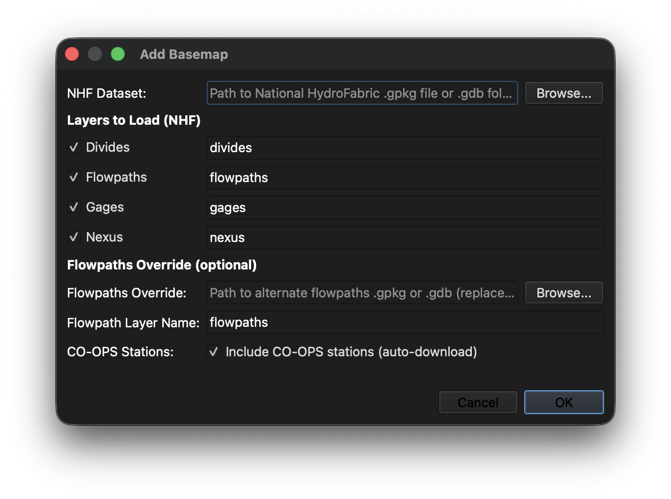
Click Add Basemap (first plugin icon). Point the dialog at the National HydroFabric .gpkg (or .gdb) for this region. Tick the layers you need (Divides, Flowpaths, Gages, Nexus) and check Include CO-OPS stations to also auto-download nearby NOAA tide gauges. An optional Flowpaths Override lets you swap in an alternate flowpaths source without re-staging the whole NHF dataset.

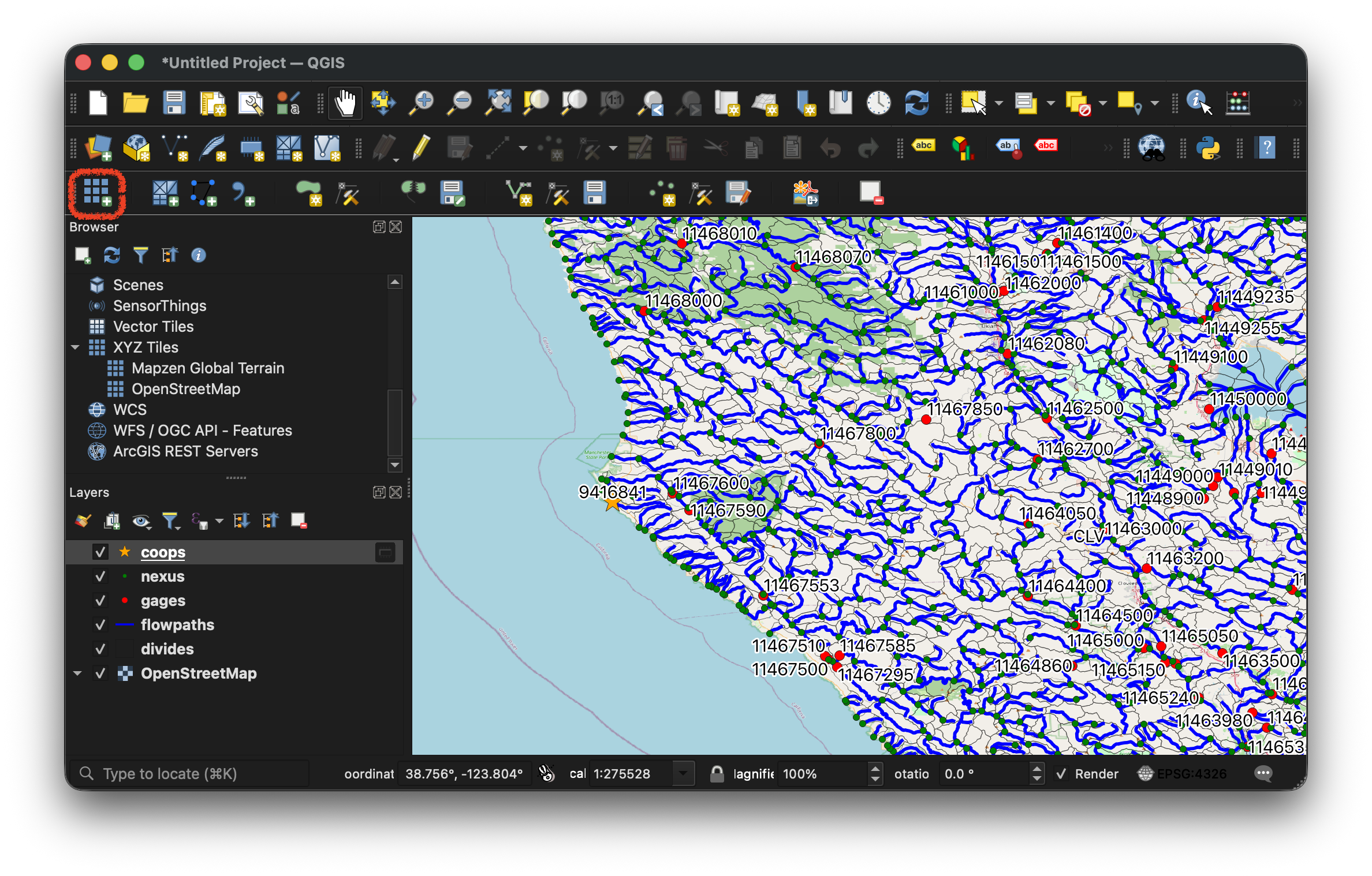
The plugin loads each layer with default styling: flowpaths in blue, divides in light yellow, gages and nexus as point layers, CO-OPS gauges as orange stars, over an OpenStreetMap base.

Step 3: Load the Pacific SCHISM mesh¶

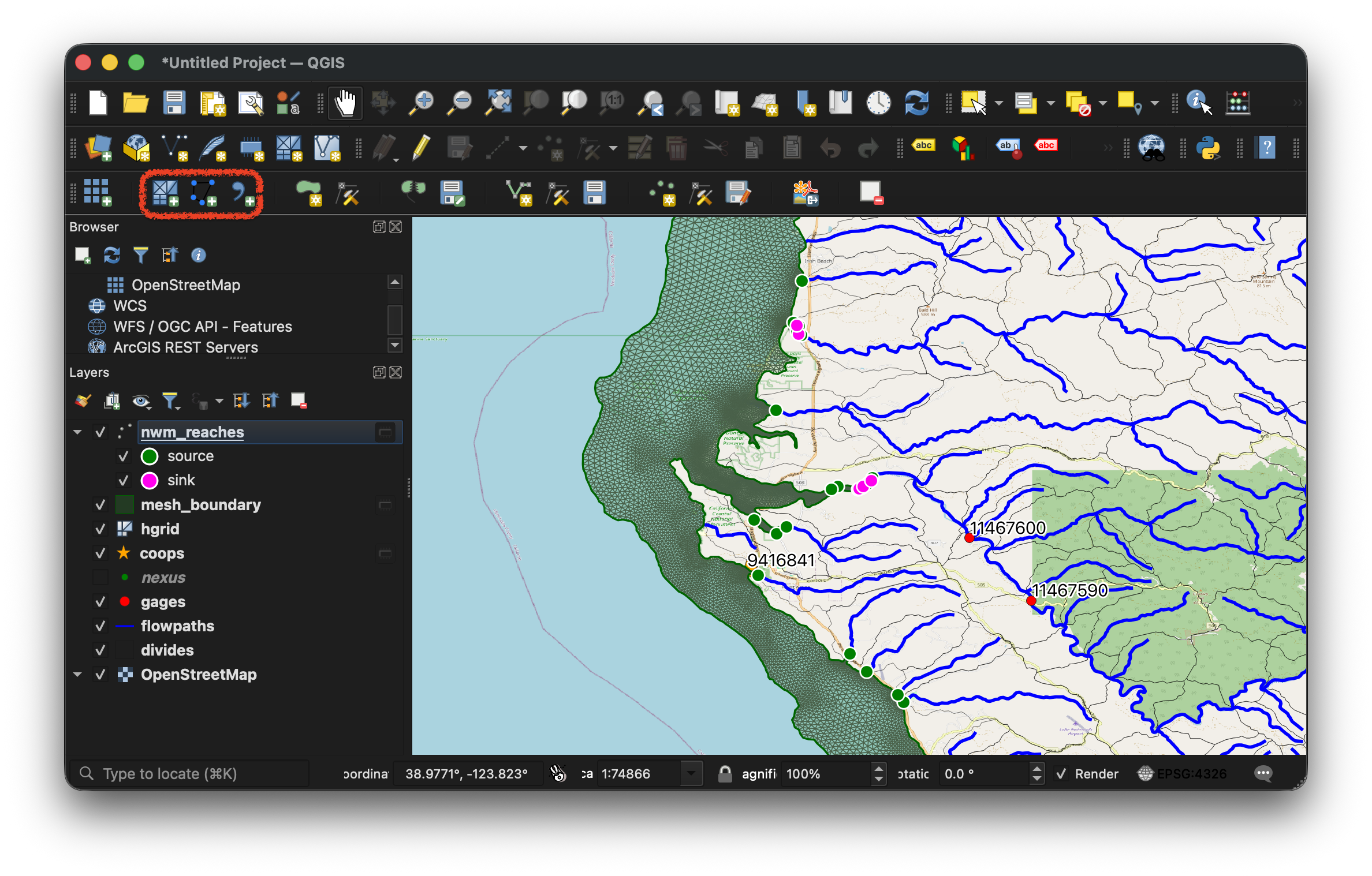
Click Load SCHISM Mesh and select the full Pacific mesh hgrid.gr3. The plugin streams the mesh into QGIS as the hgrid triangular mesh layer over the NHF basemap.

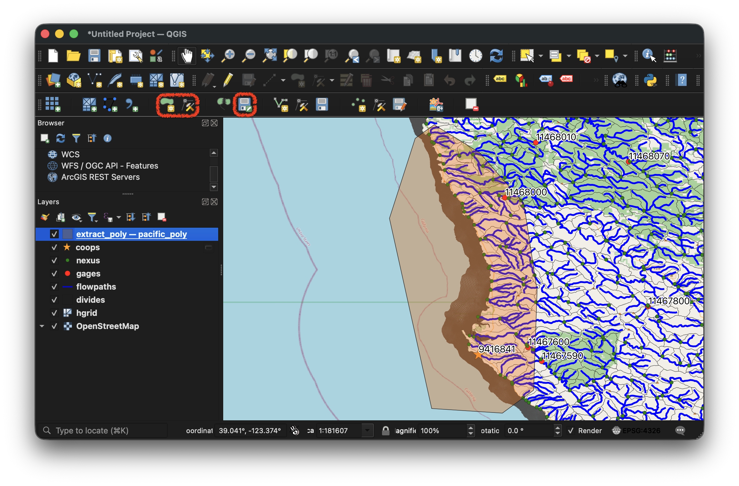
Step 4: Draw and save the subset polygon¶

Zoom into the coastal area of interest (here, the Mendocino / Point Arena coast). Click Draw Polygon from the plugin toolbar, then click on the map to place vertices that bound the subset, and double-click to finish the polygon. With the new polygon layer selected, click Save Polygon from the plugin to write extract_poly.geojson into the walkthrough directory (WGS84). The SCHISM pipeline in the next section reads this file directly.

2. Extract a SCHISM subdomain¶

extract_mesh keeps the portion of the full Pacific SCHISM mesh that falls inside the polygon and rebuilds the open boundaries where the polygon edge crosses the mesh. The result is a small, self-contained project under extracted/ ready for the pipeline runner.

In [2]:

import shapely

import coastal_calibration.schism.subsetter as ss

poly = shapely.get_geometry(shapely.from_geojson(Path("extract_poly.geojson").read_text()), 0)
print(f"Polygon: {poly.geom_type}, bounds={[round(b, 3) for b in poly.bounds]}")

res = ss.extract_mesh("model", poly, ".", output_name="extracted")
print(
    f"Extracted: {res.classification.n_side_a:,} nodes, {res.subset.side_a.n_elements:,} elements"
)

import shapely import coastal_calibration.schism.subsetter as ss poly = shapely.get_geometry(shapely.from_geojson(Path("extract_poly.geojson").read_text()), 0) print(f"Polygon: {poly.geom_type}, bounds={[round(b, 3) for b in poly.bounds]}") res = ss.extract_mesh("model", poly, ".", output_name="extracted") print( f"Extracted: {res.classification.n_side_a:,} nodes, {res.subset.side_a.n_elements:,} elements" )

Polygon: Polygon, bounds=[-123.856, 38.819, -123.616, 39.289]

Extracted: 16,508 nodes, 30,213 elements

Run the SCHISM pipeline¶

The runner executes the 12 stages: download, sflux, atmospheric regridding, boundary conditions, NWM discharge, mesh partitioning, SCHISM execution, and post-processing (station comparison + obs-points extraction). On this machine the full 50-hour simulation completes in roughly 4 minutes.

In [3]:

from coastal_calibration import CoastalCalibConfig, CoastalCalibRunner, configure_logger

configure_logger(level="INFO")

schism_run_dir = walkthrough_dir / "run_schism"

schism_config = CoastalCalibConfig.from_dict(
    {
        "model": "schism",
        "simulation": {
            "start_date": "2025-11-26",
            "duration_hours": 50,
            "coastal_domain": "pacific",
            "meteo_source": "nwm_ana",
        },
        "boundary": {"source": "stofs"},
        "paths": {
            "work_dir": str(schism_run_dir),
            "raw_download_dir": "../downloads",
        },
        "download": {"enabled": True},
        "model_config": {
            "prebuilt_dir": "./extracted",
            "geogrid_file": "./geo_em_CONUS.nc",
            "discharge_file": "./extracted/nwmReaches.csv",
            "nodes": 1,
            "ntasks_per_node": 8,
            "nscribes": 2,
            "oversubscribe": True,
            "include_noaa_gages": True,
        },
    }
)

schism_result = CoastalCalibRunner(schism_config).run()
if not schism_result.success:
    raise RuntimeError(
        f"SCHISM pipeline failed at '{schism_result.stages_failed}': {schism_result.errors}"
    )
print(schism_result)

from coastal_calibration import CoastalCalibConfig, CoastalCalibRunner, configure_logger configure_logger(level="INFO") schism_run_dir = walkthrough_dir / "run_schism" schism_config = CoastalCalibConfig.from_dict( { "model": "schism", "simulation": { "start_date": "2025-11-26", "duration_hours": 50, "coastal_domain": "pacific", "meteo_source": "nwm_ana", }, "boundary": {"source": "stofs"}, "paths": { "work_dir": str(schism_run_dir), "raw_download_dir": "../downloads", }, "download": {"enabled": True}, "model_config": { "prebuilt_dir": "./extracted", "geogrid_file": "./geo_em_CONUS.nc", "discharge_file": "./extracted/nwmReaches.csv", "nodes": 1, "ntasks_per_node": 8, "nscribes": 2, "oversubscribe": True, "include_noaa_gages": True, }, } ) schism_result = CoastalCalibRunner(schism_config).run() if not schism_result.success: raise RuntimeError( f"SCHISM pipeline failed at '{schism_result.stages_failed}': {schism_result.errors}" ) print(schism_result)

========================================                                        

Coastal Calibration Workflow                                                    

Start Time: 2026-05-21 19:35:58                                                 

========================================                                        

----------------------------------------                                        

Cleaned generated files from                                                    
docs/examples/walkthrough/run_schism      

Stage: download                                                                 

Start Time: 2026-05-21 19:35:58                                                 

  Download input data (NWM, STOFS)                                              

  meteo/nwm_ana: 51/51 [OK]                                                     

  hydro/nwm: 51/51 [OK]                                                         

  coastal/stofs: 1/1 [OK]                                                       

  Total: 103/103 (failed: 0)                                                    

  Download complete. Raw files stored in                                        
docs/examples/downloads                   

  [✓] COMPLETED (0s)                                                            

----------------------------------------                                        

Stage: schism_forcing_prep                                                      

Start Time: 2026-05-21 19:35:58                                                 

  Prepare LDASIN forcing data                                                   

  Creating forcing symlinks and output directories                              

    Staged LDASIN files in                                                      
docs/examples/walkthrough/run_schism/forci
ng_input/2025112600 (50 hours from 2025112600)                                  

  Pre-forcing complete. Output dir:                                             
docs/examples/walkthrough/run_schism/coast
al_forcing_output                                                               

  [✓] COMPLETED (0s)                                                            

----------------------------------------                                        

Stage: schism_forcing                                                           

Start Time: 2026-05-21 19:35:58                                                 

  Regrid atmospheric forcing (MPI)                                              

  Generating 50h forcing from 202511260000 via MPI                              

  NWM forcing generated in                                                      
docs/examples/walkthrough/run_schism/forci
ng_input                                                                        

  [✓] COMPLETED (21s)                                                           

----------------------------------------                                        

Stage: schism_sflux                                                             

Start Time: 2026-05-21 19:36:19                                                 

  Generate sflux atmospheric files                                              

  Generating sflux from LDASIN files                                            

    Subsetting sflux to hgrid.ll extent: (-123.810144, 38.832091, -123.638817,  
39.276069)                                                                      

    Subsetting geogrid to mesh bbox: ny 3840→179, nx 4608→144                   

    Creating sflux from 51 LDASIN files in                                      
docs/examples/walkthrough/run_schism/forci
ng_input/2025112600                                                             

    Renamed sflux_air_1.0001.nc → sflux_air_1.1.nc                              

    Generated sflux in                                                          
docs/examples/walkthrough/run_schism/sflux

  Post-processing complete. 2 sflux file(s) produced.                           

  [✓] COMPLETED (48s)                                                           

----------------------------------------                                        

Stage: schism_params                                                            

Start Time: 2026-05-21 19:37:08                                                 

  Create param.nml and symlink mesh files                                       

  Creating param.nml and symlinking mesh files                                  

    Created param.nml and symlinked mesh files in                               
docs/examples/walkthrough/run_schism      

  Parameter file created:                                                       
docs/examples/walkthrough/run_schism/param
.nml                                                                            

  [✓] COMPLETED (0s)                                                            

----------------------------------------                                        

Stage: schism_obs                                                               

Start Time: 2026-05-21 19:37:08                                                 

  Add NOAA observation stations for SCHISM                                      

  hgrid.gr3: 16508 nodes, 30213 elements                                        

  Found 3 open boundary segment(s) with 466 total nodes                         

  Loading cached station metadata from cache/coops_stations_metadata.json       

  Fetching datum information for 1 station(s)                                   

  Fetching data from 1 station(s)                                               

  station.in written with 1 NOAA station(s): 9416841                            

  [✓] COMPLETED (0s)                                                            

----------------------------------------                                        

Stage: schism_boundary                                                          

Start Time: 2026-05-21 19:37:09                                                 

  Generate boundary conditions                                                  

  Auto-resolved STOFS file:                                                     
docs/examples/downloads/coastal/stofs/stof
s_2d_glo.20251126/stofs_2d_glo.t00z.fields.cwl.nc                               

  Using STOFS file:                                                             
docs/examples/downloads/coastal/stofs/stof
s_2d_glo.20251126/stofs_2d_glo.t00z.fields.cwl.nc                               

    STOFS boundary created:                                                     
docs/examples/walkthrough/run_schism/elev2
D.th.nc                                                                         

  STOFS boundary file created:                                                  
docs/examples/walkthrough/run_schism/elev2
D.th.nc                                                                         

  [✓] COMPLETED (21s)                                                           

----------------------------------------                                        

Stage: schism_discharge                                                         

Start Time: 2026-05-21 19:37:30                                                 

  Generate river discharge forcing                                              

  Copying discharge file:                                                       
docs/examples/walkthrough/extracted/nwmRea
ches.csv                                                                        

  Symlinking NWM CHRTOUT files                                                  

  Running make_discharge                                                        

    Processing 51 CHRTOUT files                                                 

    Wrote vsource.th (51 rows), vsink.th, source_sink.in (53 sources, 20 sinks) 

  Running combine_sink_source                                                   

    combine_sink_source completed                                               

  Running merge_source_sink                                                     

    Wrote source.nc: 19 sources (from 19), 20 sinks, 51 timesteps               

  Discharge generation complete                                                 

  [✓] COMPLETED (3s)                                                            

----------------------------------------                                        

Stage: schism_prep                                                              

Start Time: 2026-05-21 19:37:34                                                 

  Partition mesh and finalize inputs                                            

  Partitioning for 8 tasks (2 scribes)                                          

    Partitioned mesh into 6 compute ranks →                                     
docs/examples/walkthrough/run_schism/parti
tion.prop                                                                       

  Set iout_sta = 1, nspool_sta = 18 in param.nml                                

  SCHISM pre-processing complete                                                

  [✓] COMPLETED (0s)                                                            

----------------------------------------                                        

Stage: schism_run                                                               

Start Time: 2026-05-21 19:37:34                                                 

  Run SCHISM model (MPI)                                                        

  Launching pschism with 8 MPI tasks (1 node(s), 2 scribe(s))                   

  Command: mpiexec -n 8 --oversubscribe                                         
.pixi/envs/dev/bin/pschism 2              

  SCHISM run completed successfully                                             

  [✓] COMPLETED (39s)                                                           

----------------------------------------                                        

Stage: schism_postprocess                                                       

Start Time: 2026-05-21 19:38:14                                                 

  Post-process SCHISM outputs                                                   

  SCHISM post-processing complete                                               

  [✓] COMPLETED (0s)                                                            

----------------------------------------                                        

Stage: schism_plot                                                              

Start Time: 2026-05-21 19:38:14                                                 

  Plot simulated vs observed water levels (SCHISM)                              

  Loading cached station metadata from cache/coops_stations_metadata.json       

  Applied per-station datum offset to simulated values (range -0.9336 to -0.9336
m, mean -0.9336 m)                                                              

  Loading cached station metadata from cache/coops_stations_metadata.json       

  Requesting water_level data for 1 station(s) from 20251126 00:00 to 20251128  
02:00                                                                           

  Fetching data from 1 station(s)                                               

  Successfully retrieved data for 1 station(s)                                  

  Loading cached station metadata from cache/coops_stations_metadata.json       

  Fetching datum information for 1 station(s)                                   

  Fetching data from 1 station(s)                                               

  Saved 1 comparison figure(s) to                                               
docs/examples/walkthrough/run_schism/figs 

  Including 1 NOAA gauge(s) from station.in                                     

  Wrote obs_water_level.parquet with 1 station(s) and 50 timestep(s)            

  [✓] COMPLETED (2s)                                                            

----------------------------------------                                        

========================================                                        

Workflow COMPLETED | Total Duration: 0:02:18                                    

========================================                                        

Timing Summary:                                                                 

----------------------------------------                                        

  [✓] download: 0s                                                              

  [✓] schism_forcing_prep: 0s                                                   

  [✓] schism_forcing: 21s                                                       

  [✓] schism_sflux: 48s                                                         

  [✓] schism_params: 0s                                                         

  [✓] schism_obs: 0s                                                            

  [✓] schism_boundary: 21s                                                      

  [✓] schism_discharge: 3s                                                      

  [✓] schism_prep: 0s                                                           

  [✓] schism_run: 39s                                                           

  [✓] schism_postprocess: 0s                                                    

  [✓] schism_plot: 2s                                                           

WorkflowResult: SUCCESS
  Start:     2026-05-21 19:35:58
  End:       2026-05-21 19:38:16
  Duration:  2m 18s
  Completed: download, schism_forcing_prep, schism_forcing, schism_sflux, schism_params, schism_obs, schism_boundary, schism_discharge, schism_prep, schism_run, schism_postprocess, schism_plot

3. QGIS plugin: derive the SFINCS AOI and discharge flowlines¶

With the SCHISM subset built and run, return to QGIS to produce the two SFINCS-side inputs:

1. aoi.geojson: a polygon that aligns the seaward edge of the SFINCS domain with the SCHISM mesh boundary and snaps the landward edge to NHF watershed divides.
2. discharge_nwm.geojson: the NWM flowlines that cross the AOI boundary, keyed by an integer NWM feature ID (column name passed to the SFINCS create stage as nwm_id_column; the create stage normalizes it to "name" internally so the run stage can look up NWM streamflow regardless of the source column name).

The walkthrough has both files pre-staged in docs/examples/walkthrough/, so Sections 4-6 are runnable today. The steps below document how those files were produced.

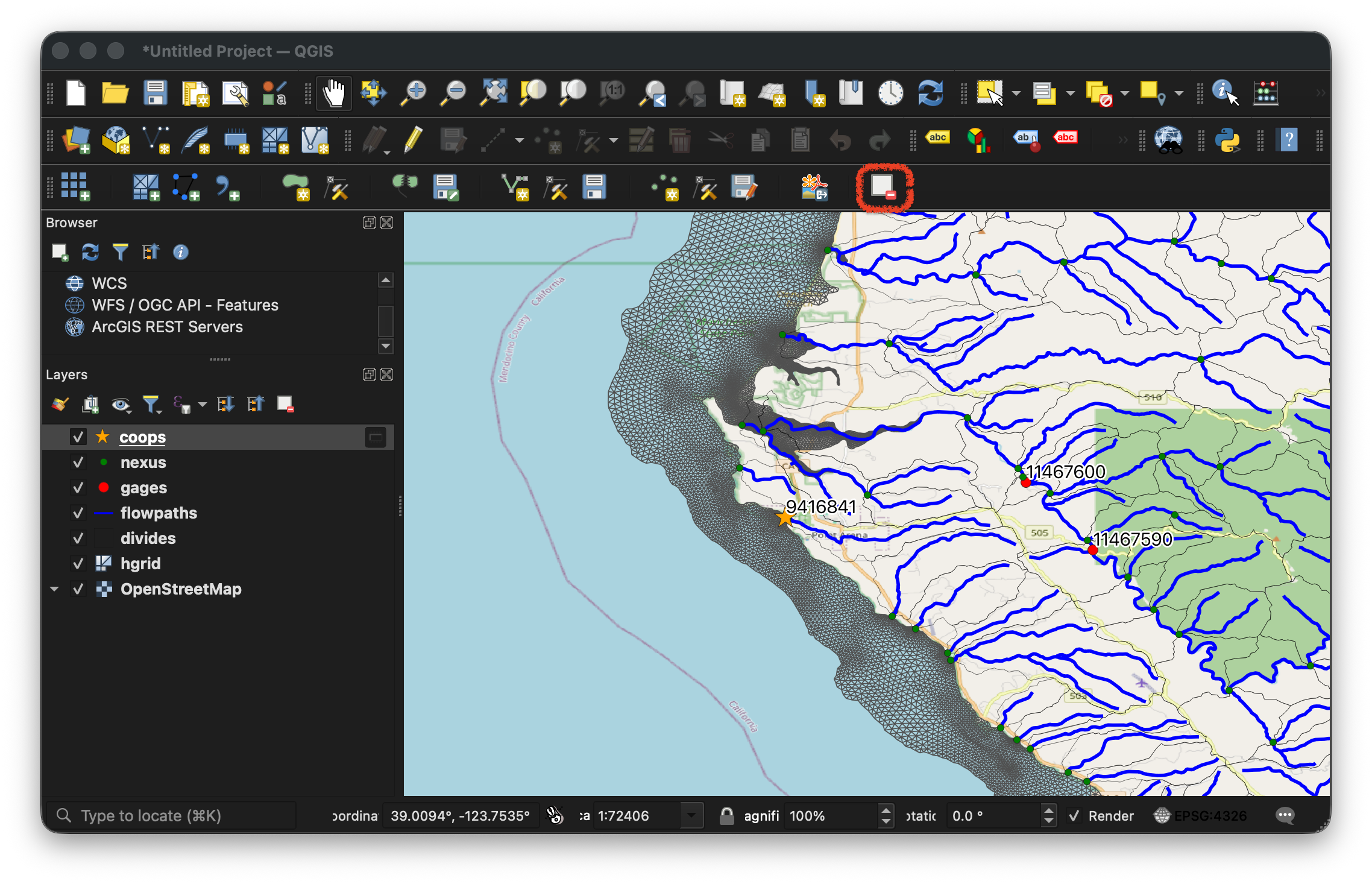
Step 1: Clear the map¶

The QGIS session from Section 1 still has the full Pacific SCHISM mesh and other intermediate layers loaded. Click Clear Map from the plugin to drop the SCHISM-related layers and leave only the NHF basemap behind, giving a clean slate for the SFINCS-side work.

Step 2: Load the subset SCHISM mesh¶

Click Load SCHISM Mesh and select extracted/hgrid.gr3 from this walkthrough directory. The plugin loads the subset mesh as the hgrid triangular mesh layer over the NHF basemap.

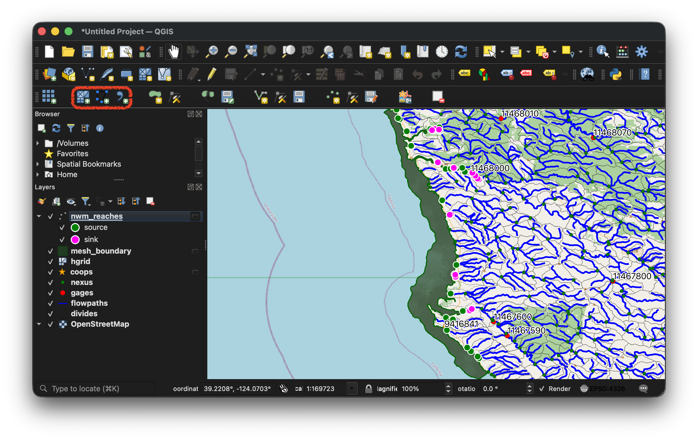
Step 3: Extract the mesh boundary and load NWM reaches¶

Click Extract Mesh Boundary. The plugin parses the open, exterior, and island boundaries from hgrid.gr3 and adds a mesh_boundary polygon layer that traces the SCHISM domain edge exactly. This polygon is the seaward seed for the SFINCS AOI.

Then click Load NWM Reaches from the plugin. This adds the sink and source points of the subset SCHISM model as a visual guide for which NWM reaches enter and leave the domain, helping you pick the right flowpaths in Step 6 below.

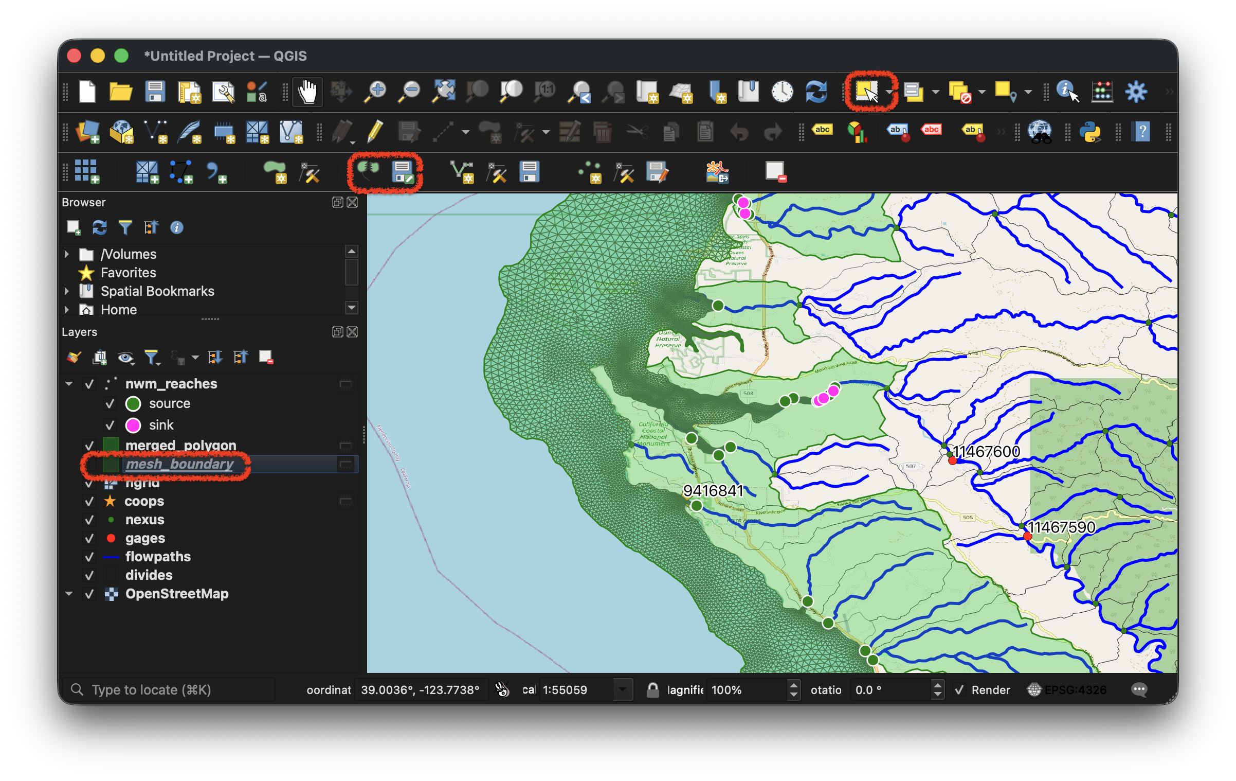
Step 4: Union the boundary with NHF divides and save the AOI¶

In the QGIS Layers panel, select the mesh_boundary layer. Use the QGIS Select Features tool to click on and select the polygon on the map. With the polygon selected, click NHF Union from the plugin. The plugin extends the boundary inland to fully include every NHF watershed divide it clips, producing a merged_polygon layer. This is what makes the SFINCS domain hydrologically meaningful: every river entering the domain has its full upstream catchment inside the AOI, so NWM discharge sources line up with watershed boundaries. With the merged_polygon layer selected and its polygon selected on the map, click Save Polygon from the plugin to write aoi.geojson (WGS84) into the walkthrough directory.

Step 5: Select and export discharge flowpaths¶

Select the flowpaths layer in the Layers panel. With the QGIS Select Features tool, select every river that crosses the AOI boundary (the NWM sink/source points loaded in Step 3 show you which ones enter or exit the domain). Once the right flowpaths are selected, click Export Selected Flowpaths from the plugin and save as discharge_nwm.geojson. The file keeps the source NHF integer ID column (ID for the demo dataset), which is what the SFINCS create stage uses to map flowlines back to NWM streamflow.

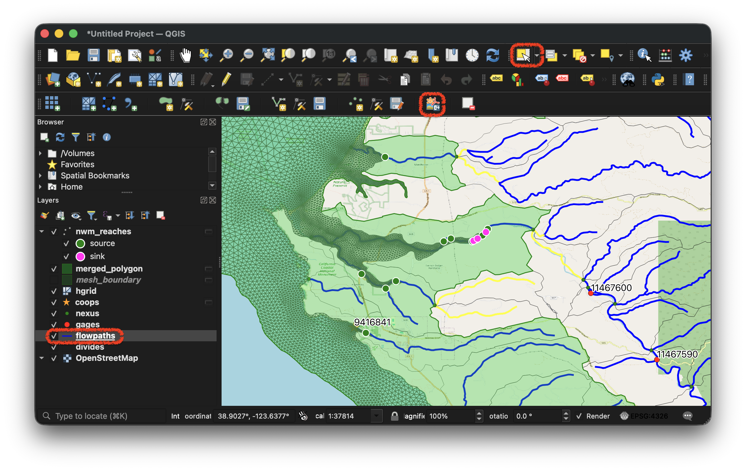
The setup cell at the top of this notebook expects extract_poly.geojson, aoi.geojson, and discharge_nwm.geojson to live in docs/examples/walkthrough/. All three are committed alongside the notebook so this section can be skipped end-to-end on a re-run. To use a different domain, regenerate them with the steps above and drop them into the walkthrough directory under the same names.

4. Build & run the SFINCS model¶

SfincsCreateConfig.from_dict bundles every input the model needs: the AOI polygon, a base 512 m quadtree grid with one refinement level inside the AOI, NOAA CRM 3 arc-second (~90 m) topobathy + GEBCO elevation, ESA WorldCover-derived Manning's n, and the QGIS-derived flowlines as discharge sources. CRM is a public, integrated topobathy product from NCEI THREDDS, and it resolves coastal bays that the land-only Copernicus DEM misses. add_noaa_gages: True also auto-discovers the same NOAA tide gauge the SCHISM pipeline uses, which is what makes the 3-line comparison in Part 4 work without any manual station bookkeeping.

In [4]:

from coastal_calibration import SfincsCreateConfig, SfincsCreator

create_config = SfincsCreateConfig.from_dict(
    {
        "aoi": "./aoi.geojson",
        "output_dir": "./output_sfincs",
        "download_dir": "../downloads/walkthrough_grid",
        "grid": {
            "resolution": 512,
            "crs": "utm",
            "rotated": False,
            # Refine along the coast (SCHISM mesh boundary) rather than
            # the full NHF-union AOI: the coastal corridor is where
            # SFINCS needs higher resolution to keep narrow connections
            # wet across the tidal cycle. Level 4 = 32 m cells.
            "refinement": [
                {"polygon": "./refine_poly.geojson", "level": 4, "buffer_m": -200},
            ],
        },
        "elevation": {
            "datasets": [
                {
                    "name": "noaa_crm",
                    "zmin": -20000,
                    "source": "noaa_crm",
                },
                {"name": "gebco_15arcs", "zmin": -20000, "source": "gebco_15arcs"},
            ],
            "buffer_cells": 1,
        },
        "mask": {
            "zmin": -50.0,
            "boundary_zmax": -1.0,
            "reset_bounds": True,
            # Drop tiny isolated active cells just above zmin (offshore
            # bumps that clear the -50 m cutoff but are surrounded by
            # deeper inactive cells) so the model is a single connected
            # domain instead of a few floating fragments.
            "keep_largest_only": True,
        },
        "subgrid": {
            "nr_subgrid_pixels": 4,
            "lulc_dataset": "esa_worldcover",
            "manning_land": 0.04,
            "manning_sea": 0.02,
        },
        "river_discharge": {
            "flowlines": "./discharge_nwm.geojson",
            # `nwm_reaches.geojson` from the QGIS plugin uses "ID" for the
            # NWM feature ID; create.py renames it to "name" internally so
            # the run stage's NWM streamflow lookup works regardless.
            "nwm_id_column": "ID",
        },
        "add_noaa_gages": True,
    }
)

create_result = SfincsCreator(create_config).run()
if not create_result.success:
    raise RuntimeError(
        f"SFINCS create failed at '{create_result.stages_failed}': {create_result.errors}"
    )
print(create_result)

from coastal_calibration import SfincsCreateConfig, SfincsCreator create_config = SfincsCreateConfig.from_dict( { "aoi": "./aoi.geojson", "output_dir": "./output_sfincs", "download_dir": "../downloads/walkthrough_grid", "grid": { "resolution": 512, "crs": "utm", "rotated": False, # Refine along the coast (SCHISM mesh boundary) rather than # the full NHF-union AOI: the coastal corridor is where # SFINCS needs higher resolution to keep narrow connections # wet across the tidal cycle. Level 4 = 32 m cells. "refinement": [ {"polygon": "./refine_poly.geojson", "level": 4, "buffer_m": -200}, ], }, "elevation": { "datasets": [ { "name": "noaa_crm", "zmin": -20000, "source": "noaa_crm", }, {"name": "gebco_15arcs", "zmin": -20000, "source": "gebco_15arcs"}, ], "buffer_cells": 1, }, "mask": { "zmin": -50.0, "boundary_zmax": -1.0, "reset_bounds": True, # Drop tiny isolated active cells just above zmin (offshore # bumps that clear the -50 m cutoff but are surrounded by # deeper inactive cells) so the model is a single connected # domain instead of a few floating fragments. "keep_largest_only": True, }, "subgrid": { "nr_subgrid_pixels": 4, "lulc_dataset": "esa_worldcover", "manning_land": 0.04, "manning_sea": 0.02, }, "river_discharge": { "flowlines": "./discharge_nwm.geojson", # `nwm_reaches.geojson` from the QGIS plugin uses "ID" for the # NWM feature ID; create.py renames it to "name" internally so # the run stage's NWM streamflow lookup works regardless. "nwm_id_column": "ID", }, "add_noaa_gages": True, } ) create_result = SfincsCreator(create_config).run() if not create_result.success: raise RuntimeError( f"SFINCS create failed at '{create_result.stages_failed}': {create_result.errors}" ) print(create_result)

========================================                                        

Coastal Calibration Workflow                                                    

Start Time: 2026-05-21 19:38:18                                                 

========================================                                        

----------------------------------------                                        

Stage: create_grid                                                              

Start Time: 2026-05-21 19:38:18                                                 

  Create SFINCS grid from AOI                                                   

  AOI:                                                                          
docs/examples/walkthrough/aoi.geojson     

  Resolution: 512 m, CRS: utm                                                   

  Refinement polygon 'refine_poly.geojson': split into 2 component(s) after     
buffer_m=-200 m                                                                 

  Refinement: 1 polygon(s), max level 4                                         

  Grid created successfully                                                     

  [✓] COMPLETED (3s)                                                            

----------------------------------------                                        

Stage: create_fetch_data                                                        

Start Time: 2026-05-21 19:38:21                                                 

  Fetch elevation and land cover data for AOI                                   

  Reusing existing noaa_crm.tif                                                 

  Reusing existing gebco_15arcs.tif                                             

  Reusing existing esa_worldcover.tif                                           

  Fetched 3 dataset(s): ['noaa_crm', 'gebco_15arcs', 'esa_worldcover']          

  [✓] COMPLETED (0s)                                                            

----------------------------------------                                        

Stage: create_elevation                                                         

Start Time: 2026-05-21 19:38:21                                                 

  Add elevation and bathymetry data                                             

  Elevation datasets: ['noaa_crm', 'gebco_15arcs']                              

  Elevation created successfully                                                

  [✓] COMPLETED (0s)                                                            

----------------------------------------                                        

Stage: create_mask                                                              

Start Time: 2026-05-21 19:38:22                                                 

  Create active cell mask                                                       

  zmin=-50.0                                                                    

  Active mask created successfully                                              

  [✓] COMPLETED (0s)                                                            

----------------------------------------                                        

Stage: create_boundary                                                          

Start Time: 2026-05-21 19:38:22                                                 

  Create water level boundary cells                                             

  boundary_zmax=-1.0                                                            

  Boundary cells created successfully                                           

  [✓] COMPLETED (0s)                                                            

----------------------------------------                                        

Stage: create_discharge                                                         

Start Time: 2026-05-21 19:38:22                                                 

  Add river discharge source points                                             

  Read 26 flowpath(s) from discharge_nwm.geojson                                

    2666131: snapped to active cell (103 m away)                                

    2666047: snapped to active cell (215 m away)                                

    2665943: snapped to active cell (227 m away)                                

    2664809: snapped to active cell (135 m away)                                

    2664713: snapped to active cell (140 m away)                                

    2664573: snapped to active cell (160 m away)                                

    2664269: snapped to active cell (187 m away)                                

    2664215: snapped to active cell (217 m away)                                

    2664367: snapped to active cell (291 m away)                                

    2664397: snapped to active cell (269 m away)                                

    2664659: snapped to active cell (120 m away)                                

    2665573: snapped to active cell (123 m away)                                

    2664447: snapped to active cell (241 m away)                                

    2664465: snapped to active cell (241 m away)                                

    2664753: snapped to active cell (144 m away)                                

    2664899: snapped to active cell (63 m away)                                 

    2664951: snapped to active cell (35 m away)                                 

    2666173: snapped to active cell (238 m away)                                

    2666193: snapped to active cell (208 m away)                                

    2664551: snapped to active cell (160 m away)                                

    2664761: snapped to active cell (147 m away)                                

    2664993: snapped to active cell (42 m away)                                 

    2665043: snapped to active cell (72 m away)                                 

    2665949: snapped to active cell (227 m away)                                

    2666017: snapped to active cell (215 m away)                                

    2666079: snapped to active cell (99 m away)                                 

  Wrote 26 discharge source location(s) to sfincs_nwm.src                       

  [✓] COMPLETED (0s)                                                            

----------------------------------------                                        

Stage: create_subgrid                                                           

Start Time: 2026-05-21 19:38:23                                                 

  Create subgrid tables                                                         

  nr_subgrid_pixels=4                                                           

  Subgrid tables created successfully                                           

  [✓] COMPLETED (20s)                                                           

----------------------------------------                                        

Stage: create_obs                                                               

Start Time: 2026-05-21 19:38:43                                                 

  Add observation points                                                        

  Loading cached station metadata from cache/coops_stations_metadata.json       

  Fetching datum information for 1 station(s)                                   

  Fetching data from 1 station(s)                                               

  Added 1 NOAA CO-OPS observation point(s)                                      

    noaa_9416841: placed at face center z=-3.186 m (51 m from original)         

  Snapped 1 observation point(s) to nearest wet cell                            

  [✓] COMPLETED (0s)                                                            

----------------------------------------                                        

Stage: create_write                                                             

Start Time: 2026-05-21 19:38:43                                                 

  Write SFINCS model to disk                                                    

  Output directory:                                                             
docs/examples/walkthrough/output_sfincs   

  Model written successfully                                                    

  [✓] COMPLETED (0s)                                                            

----------------------------------------                                        

========================================                                        

Workflow COMPLETED | Total Duration: 0:00:25                                    

========================================                                        

Timing Summary:                                                                 

----------------------------------------                                        

  [✓] create_grid: 3s                                                           

  [✓] create_fetch_data: 0s                                                     

  [✓] create_elevation: 0s                                                      

  [✓] create_mask: 0s                                                           

  [✓] create_boundary: 0s                                                       

  [✓] create_discharge: 0s                                                      

  [✓] create_subgrid: 20s                                                       

  [✓] create_obs: 0s                                                            

  [✓] create_write: 0s                                                          

WorkflowResult: SUCCESS
  Start:     2026-05-21 19:38:18
  End:       2026-05-21 19:38:43
  Duration:  25s
  Completed: create_grid, create_fetch_data, create_elevation, create_mask, create_boundary, create_discharge, create_subgrid, create_obs, create_write

In [5]:

sfincs_run_dir = walkthrough_dir / "run_sfincs"

sfincs_run_config = CoastalCalibConfig.from_dict(
    {
        "model": "sfincs",
        "simulation": {
            "start_date": "2025-11-26",
            "duration_hours": 50,
            "coastal_domain": "pacific",
            "meteo_source": "nwm_ana",
        },
        "boundary": {"source": "stofs"},
        "paths": {
            "work_dir": str(sfincs_run_dir),
            "raw_download_dir": "../downloads",
        },
        "download": {"enabled": True},
        "model_config": {
            "prebuilt_dir": "./output_sfincs",
            "discharge_locations_file": "./output_sfincs/sfincs_nwm.src",
            "merge_discharge": True,
            "forcing_to_mesh_offset_m": 0.0,
            # NAVD88→LMSL offset for Mendocino (~39N, -123.7W) from NOAA VDatum.
            # Verify / re-derive for other domains via:
            # https://vdatum.noaa.gov/vdatumweb/api/convert?s_x=<lon>&s_y=<lat>&s_z=0&region=westcoast&s_h_frame=NAD83_2011&s_v_frame=NAVD88&t_h_frame=IGS14&t_v_frame=LMSL
            "vdatum_mesh_to_msl_m": -0.92,
            "include_precip": True,
            "include_wind": True,
            "include_pressure": True,
            "floodmap_dem": "../downloads/walkthrough_grid/noaa_crm.tif",
            # Stability settings tuned for tidal + compound flooding on a
            # finely refined coastal mesh. ``advection=0`` is the
            # standard SFINCS choice for tide-dominated runs (advection
            # destabilises shallow water at low tide on quadtree
            # transitions); a small constant viscosity damps residual
            # high-frequency noise. Same family of settings as the
            # Lavaca demo (``docs/examples/notebooks/lavaca.py``).
            "run_param_overrides": {
                "tspinup": 10800,
                "advection": 0,
                "viscosity": 0,
                "nuvisc": 0.01,
            },
        },
    }
)

sfincs_result = CoastalCalibRunner(sfincs_run_config).run()
if not sfincs_result.success:
    raise RuntimeError(
        f"SFINCS pipeline failed at '{sfincs_result.stages_failed}': {sfincs_result.errors}"
    )
print(sfincs_result)

sfincs_run_dir = walkthrough_dir / "run_sfincs" sfincs_run_config = CoastalCalibConfig.from_dict( { "model": "sfincs", "simulation": { "start_date": "2025-11-26", "duration_hours": 50, "coastal_domain": "pacific", "meteo_source": "nwm_ana", }, "boundary": {"source": "stofs"}, "paths": { "work_dir": str(sfincs_run_dir), "raw_download_dir": "../downloads", }, "download": {"enabled": True}, "model_config": { "prebuilt_dir": "./output_sfincs", "discharge_locations_file": "./output_sfincs/sfincs_nwm.src", "merge_discharge": True, "forcing_to_mesh_offset_m": 0.0, # NAVD88→LMSL offset for Mendocino (~39N, -123.7W) from NOAA VDatum. # Verify / re-derive for other domains via: # https://vdatum.noaa.gov/vdatumweb/api/convert?s_x=<lon>&s_y=<lat>&s_z=0&region=westcoast&s_h_frame=NAD83_2011&s_v_frame=NAVD88&t_h_frame=IGS14&t_v_frame=LMSL "vdatum_mesh_to_msl_m": -0.92, "include_precip": True, "include_wind": True, "include_pressure": True, "floodmap_dem": "../downloads/walkthrough_grid/noaa_crm.tif", # Stability settings tuned for tidal + compound flooding on a # finely refined coastal mesh. ``advection=0`` is the # standard SFINCS choice for tide-dominated runs (advection # destabilises shallow water at low tide on quadtree # transitions); a small constant viscosity damps residual # high-frequency noise. Same family of settings as the # Lavaca demo (``docs/examples/notebooks/lavaca.py``). "run_param_overrides": { "tspinup": 10800, "advection": 0, "viscosity": 0, "nuvisc": 0.01, }, }, } ) sfincs_result = CoastalCalibRunner(sfincs_run_config).run() if not sfincs_result.success: raise RuntimeError( f"SFINCS pipeline failed at '{sfincs_result.stages_failed}': {sfincs_result.errors}" ) print(sfincs_result)

========================================                                        

Coastal Calibration Workflow                                                    

Start Time: 2026-05-21 19:38:43                                                 

========================================                                        

----------------------------------------                                        

Cleaned generated files from                                                    
docs/examples/walkthrough/run_sfincs      

Stage: download                                                                 

Start Time: 2026-05-21 19:38:43                                                 

  Download input data (NWM, STOFS)                                              

  meteo/nwm_ana: 51/51 [OK]                                                     

  hydro/nwm: 51/51 [OK]                                                         

  coastal/stofs: 1/1 [OK]                                                       

  Total: 103/103 (failed: 0)                                                    

  Download complete. Raw files stored in                                        
docs/examples/downloads                   

  [✓] COMPLETED (0s)                                                            

----------------------------------------                                        

Stage: sfincs_symlinks                                                          

Start Time: 2026-05-21 19:38:43                                                 

  Create .nc symlinks for NWM data                                              

  Skipped 213 meteo + 0 streamflow symlinks (already exist)                     

  [✓] COMPLETED (0s)                                                            

----------------------------------------                                        

Stage: sfincs_data_catalog                                                      

Start Time: 2026-05-21 19:38:43                                                 

  Generate HydroMT data catalog for SFINCS                                      

  Data catalog written to                                                       
docs/examples/walkthrough/run_sfincs/data_
catalog.yml                                                                     

  [✓] COMPLETED (0s)                                                            

----------------------------------------                                        

Stage: sfincs_init                                                              

Start Time: 2026-05-21 19:38:43                                                 

  Initialize SFINCS model (pre-built)                                           

  Copied pre-built model from                                                   
docs/examples/walkthrough/output_sfincs to
docs/examples/walkthrough/run_sfincs/sfinc
s_model                                                                         

  Removed stale output files: sfincs_netbndbzsbzifile.nc, sfincs_netamuv.nc,    
sfincs_netamp.nc, sfincs_netampr.nc, sfincs_map.nc, sfincs_his.nc               

  SFINCS model initialized (grid_type=quadtree) at                              
docs/examples/walkthrough/run_sfincs/sfinc
s_model                                                                         

  [✓] COMPLETED (0s)                                                            

----------------------------------------                                        

Stage: sfincs_timing                                                            

Start Time: 2026-05-21 19:38:44                                                 

  Set SFINCS timing                                                             

  Spinup: 3600 s                                                                

  Timing set: 2025-11-26 00:00:00 to 2025-11-28 02:00:00                        

  [✓] COMPLETED (0s)                                                            

----------------------------------------                                        

Stage: sfincs_forcing                                                           

Start Time: 2026-05-21 19:38:44                                                 

  Add water level forcing                                                       

  Read 825 boundary point(s) from                                               
docs/examples/walkthrough/run_sfincs/sfinc
s_model/sfincs.bnd                                                              

  Loaded stofs_waterlevel: time=51, node=15244                                  

  Interpolated stofs_waterlevel to 825 boundary points (51 time steps)          

  Wrote boundary forcing to sfincs_netbndbzsbzifile.nc                          

  Water level forcing added from stofs_waterlevel                               

  [✓] COMPLETED (8s)                                                            

----------------------------------------                                        

Stage: sfincs_discharge                                                         

Start Time: 2026-05-21 19:38:52                                                 

  Add discharge sources                                                         

  Added 26 discharge source point(s) from                                       
docs/examples/walkthrough/output_sfincs/sf
incs_nwm.src                                                                    

  Assigned discharge timeseries to 26 point(s) (26 unique feature_id(s))        

  [✓] COMPLETED (3s)                                                            

----------------------------------------                                        

Stage: sfincs_precip                                                            

Start Time: 2026-05-21 19:38:56                                                 

  Add precipitation forcing                                                     

  Precipitation forcing added from nwm_ana_meteo (res=512 m)                    

  [✓] COMPLETED (1s)                                                            

----------------------------------------                                        

Stage: sfincs_wind                                                              

Start Time: 2026-05-21 19:38:57                                                 

  Add wind forcing                                                              

  Wind forcing added from nwm_ana_meteo (res=512 m)                             

  [✓] COMPLETED (1s)                                                            

----------------------------------------                                        

Stage: sfincs_pressure                                                          

Start Time: 2026-05-21 19:38:59                                                 

  Add atmospheric pressure forcing                                              

  Atmospheric pressure forcing added from nwm_ana_meteo (baro=1, res=512 m)     

  [✓] COMPLETED (1s)                                                            

----------------------------------------                                        

Stage: sfincs_write                                                             

Start Time: 2026-05-21 19:39:00                                                 

  Write SFINCS model                                                            

  Applied 4 sfincs.inp override(s): {'tspinup': 10800, 'advection': 0,          
'viscosity': 0, 'nuvisc': 0.01}                                                 

  SFINCS model written to                                                       
docs/examples/walkthrough/run_sfincs/sfinc
s_model                                                                         

  [✓] COMPLETED (0s)                                                            

----------------------------------------                                        

Stage: sfincs_run                                                               

Start Time: 2026-05-21 19:39:01                                                 

  Run SFINCS model                                                              

  Running SFINCS via native executable:                                         
.pixi/envs/dev/bin/sfincs                 

  SFINCS run completed                                                          

  [✓] COMPLETED (6m 40s)                                                        

----------------------------------------                                        

Stage: sfincs_floodmap                                                          

Start Time: 2026-05-21 19:45:41                                                 

  Downscale flood depth map                                                     

  Loaded zsmax from                                                             
docs/examples/walkthrough/run_sfincs/sfinc
s_model/sfincs_map.nc                                                           

  Creating index COG:                                                           
docs/examples/walkthrough/run_sfincs/sfinc
s_model/floodmap_index.tif                                                      

  Index COG created (0.0 MB)                                                    

  Downscaling flood depth map                                                   

  GeoTIFF has no overviews, building them: floodmap_hmax.tif                    

  Building 1 overview levels: [2]                                               

  Flood depth map written:                                                      
docs/examples/walkthrough/run_sfincs/sfinc
s_model/floodmap_hmax.tif (0.1 MB)                                              

  Flood depth map:                                                              
docs/examples/walkthrough/run_sfincs/sfinc
s_model/floodmap_hmax.tif                                                       

  [✓] COMPLETED (0s)                                                            

----------------------------------------                                        

Stage: sfincs_plot                                                              

Start Time: 2026-05-21 19:45:42                                                 

  Plot simulated vs observed water levels                                       

  Loading cached station metadata from cache/coops_stations_metadata.json       

  Fetching datum information for 1 station(s)                                   

  Fetching data from 1 station(s)                                               

  Matched 1 observation point(s) to NOAA station(s): 9416841                    

  Applied mesh→MSL vdatum offset: -0.9200 m                                     

  Loading cached station metadata from cache/coops_stations_metadata.json       

  Requesting water_level data for 1 station(s) from 20251126 00:00 to 20251128  
02:00                                                                           

  Fetching data from 1 station(s)                                               

  Successfully retrieved data for 1 station(s)                                  

  Loading cached station metadata from cache/coops_stations_metadata.json       

  Fetching datum information for 1 station(s)                                   

  Fetching data from 1 station(s)                                               

  Saved 1 comparison figure(s) to                                               
docs/examples/walkthrough/run_sfincs/sfinc
s_model/figs                                                                    

  Including 1 NOAA gauge(s) from obs_station_map.json                           

  Wrote obs_water_level.parquet with 1 station(s) and 51 timestep(s)            

  [✓] COMPLETED (1s)                                                            

----------------------------------------                                        

========================================                                        

Workflow COMPLETED | Total Duration: 0:06:59                                    

========================================                                        

Timing Summary:                                                                 

----------------------------------------                                        

  [✓] download: 0s                                                              

  [✓] sfincs_symlinks: 0s                                                       

  [✓] sfincs_data_catalog: 0s                                                   

  [✓] sfincs_init: 0s                                                           

  [✓] sfincs_timing: 0s                                                         

  [✓] sfincs_forcing: 8s                                                        

  [✓] sfincs_discharge: 3s                                                      

  [✓] sfincs_precip: 1s                                                         

  [✓] sfincs_wind: 1s                                                           

  [✓] sfincs_pressure: 1s                                                       

  [✓] sfincs_write: 0s                                                          

  [✓] sfincs_run: 6m 40s                                                        

  [✓] sfincs_floodmap: 0s                                                       

  [✓] sfincs_plot: 1s                                                           

WorkflowResult: SUCCESS
  Start:     2026-05-21 19:38:43
  End:       2026-05-21 19:45:43
  Duration:  6m 59s
  Completed: download, sfincs_symlinks, sfincs_data_catalog, sfincs_init, sfincs_timing, sfincs_forcing, sfincs_discharge, sfincs_precip, sfincs_wind, sfincs_pressure, sfincs_write, sfincs_run, sfincs_floodmap, sfincs_plot

5. Compare water levels at the NOAA gauge¶

Each pipeline writes obs_water_level.parquet to its run directory, a station × time table of modeled water levels at every observation point picked up during post-processing (in this domain, just the one CO-OPS gauge that lies inside both meshes). Combined with a fresh query_coops_byids call for the matching observed series, we feed both runs into plot_station_comparison and get a single figure with Observed, SCHISM, and SFINCS lines per station.

In [6]:

from datetime import timedelta

import pandas as pd

from coastal_calibration.data.coops_api import COOPSAPIClient, query_coops_byids
from coastal_calibration.plotting import plot_station_comparison

schism_obs_parquet = schism_run_dir / "obs_water_level.parquet"
sfincs_obs_parquet = sfincs_run_dir / "sfincs_model" / "obs_water_level.parquet"

schism_series = pd.read_parquet(schism_obs_parquet)
sfincs_series = pd.read_parquet(sfincs_obs_parquet)
print(f"SCHISM obs columns: {list(schism_series.columns)}")
print(f"SFINCS obs columns: {list(sfincs_series.columns)}")

# Keep only the CO-OPS station IDs (numeric 7-digit codes).
common_stations = sorted(set(schism_series.columns) & set(sfincs_series.columns))
station_ids = [s for s in common_stations if s.isdigit() and len(s) == 7]
if not station_ids:
    raise RuntimeError(
        "No NOAA CO-OPS station appears in both runs' obs_water_level.parquet. "
        "Check that `add_noaa_gages` (SFINCS) and `include_noaa_gages` (SCHISM) "
        "both selected at least one gauge in the domain."
    )
print(f"Comparison stations: {station_ids}")

# Re-fetch CO-OPS observations for the simulation window and convert to MSL.
sim = schism_config.simulation
begin_date = sim.start_date.strftime("%Y%m%d %H:%M")
end_dt = sim.start_date + timedelta(hours=sim.duration_hours)
end_date = end_dt.strftime("%Y%m%d %H:%M")

obs_ds = query_coops_byids(
    station_ids,
    begin_date,
    end_date,
    product="water_level",
    datum="MLLW",
    units="metric",
    time_zone="gmt",
)

datums = COOPSAPIClient().get_datums(station_ids)
datum_map = {d.station_id: d for d in datums}
for sid in station_ids:
    d = datum_map.get(sid)
    if d is None:
        continue
    msl = d.get_datum_value("MSL")
    mllw = d.get_datum_value("MLLW")
    if msl is None or mllw is None:
        continue
    offset = msl - mllw
    if d.units == "feet":
        offset *= 0.3048
    obs_ds.water_level.loc[{"station": sid}] -= offset
obs_ds.attrs["datum"] = "MSL"

# Build (times, elevation[n_t, n_stations]) tuples in the column order of station_ids.
schism_pair = (
    schism_series.index.to_numpy(),
    schism_series[station_ids].to_numpy(),
)
sfincs_pair = (
    sfincs_series.index.to_numpy(),
    sfincs_series[station_ids].to_numpy(),
)

walkthrough_figs = walkthrough_dir / "figs"
walkthrough_figs.mkdir(exist_ok=True)
combined_paths = plot_station_comparison(
    {"SCHISM": schism_pair, "SFINCS": sfincs_pair},
    station_ids,
    walkthrough_figs,
    obs_ds=obs_ds,
)
print(f"Wrote {len(combined_paths)} comparison figure(s) to {walkthrough_figs}")

from datetime import timedelta import pandas as pd from coastal_calibration.data.coops_api import COOPSAPIClient, query_coops_byids from coastal_calibration.plotting import plot_station_comparison schism_obs_parquet = schism_run_dir / "obs_water_level.parquet" sfincs_obs_parquet = sfincs_run_dir / "sfincs_model" / "obs_water_level.parquet" schism_series = pd.read_parquet(schism_obs_parquet) sfincs_series = pd.read_parquet(sfincs_obs_parquet) print(f"SCHISM obs columns: {list(schism_series.columns)}") print(f"SFINCS obs columns: {list(sfincs_series.columns)}") # Keep only the CO-OPS station IDs (numeric 7-digit codes). common_stations = sorted(set(schism_series.columns) & set(sfincs_series.columns)) station_ids = [s for s in common_stations if s.isdigit() and len(s) == 7] if not station_ids: raise RuntimeError( "No NOAA CO-OPS station appears in both runs' obs_water_level.parquet. " "Check that `add_noaa_gages` (SFINCS) and `include_noaa_gages` (SCHISM) " "both selected at least one gauge in the domain." ) print(f"Comparison stations: {station_ids}") # Re-fetch CO-OPS observations for the simulation window and convert to MSL. sim = schism_config.simulation begin_date = sim.start_date.strftime("%Y%m%d %H:%M") end_dt = sim.start_date + timedelta(hours=sim.duration_hours) end_date = end_dt.strftime("%Y%m%d %H:%M") obs_ds = query_coops_byids( station_ids, begin_date, end_date, product="water_level", datum="MLLW", units="metric", time_zone="gmt", ) datums = COOPSAPIClient().get_datums(station_ids) datum_map = {d.station_id: d for d in datums} for sid in station_ids: d = datum_map.get(sid) if d is None: continue msl = d.get_datum_value("MSL") mllw = d.get_datum_value("MLLW") if msl is None or mllw is None: continue offset = msl - mllw if d.units == "feet": offset *= 0.3048 obs_ds.water_level.loc[{"station": sid}] -= offset obs_ds.attrs["datum"] = "MSL" # Build (times, elevation[n_t, n_stations]) tuples in the column order of station_ids. schism_pair = ( schism_series.index.to_numpy(), schism_series[station_ids].to_numpy(), ) sfincs_pair = ( sfincs_series.index.to_numpy(), sfincs_series[station_ids].to_numpy(), ) walkthrough_figs = walkthrough_dir / "figs" walkthrough_figs.mkdir(exist_ok=True) combined_paths = plot_station_comparison( {"SCHISM": schism_pair, "SFINCS": sfincs_pair}, station_ids, walkthrough_figs, obs_ds=obs_ds, ) print(f"Wrote {len(combined_paths)} comparison figure(s) to {walkthrough_figs}")

  Loading cached station metadata from cache/coops_stations_metadata.json       

  Requesting water_level data for 1 station(s) from 20251126 00:00 to 20251128  
02:00                                                                           

  Fetching data from 1 station(s)                                               

  Successfully retrieved data for 1 station(s)                                  

SCHISM obs columns: ['9416841']
SFINCS obs columns: ['9416841']
Comparison stations: ['9416841']

  Loading cached station metadata from cache/coops_stations_metadata.json       

  Fetching datum information for 1 station(s)                                   

  Fetching data from 1 station(s)                                               

Wrote 1 comparison figure(s) to docs/examples/walkthrough/figs

In [7]:

from IPython.display import Image, display

for png in combined_paths:
    display(Image(filename=str(png), width=900))

from IPython.display import Image, display for png in combined_paths: display(Image(filename=str(png), width=900))

6. Side-by-side spatial animation¶

animate_water_level_comparison renders two panels driven by their own datasets but locked to a shared colormap range and synchronised on a common time clock. The two models output at different cadences (SCHISM hourly, SFINCS half-hourly), so the function takes the intersection of their time coverage, picks the coarser axis as the master clock, and uses nearest-neighbour lookup to populate the other panel each frame.

A note on the river channels¶

Both models show water at the upstream NWM inflow points but not along the river course down to the ocean. This is not a bug; it is a property of the NOAA CRM topobathy DEM: at 3 arc-second (~90 m) the CRM resolves the seaward bathymetry of the bay but is still too coarse to carve narrow river channels into the inland part of the grid. The model bed along the rivers therefore sits at the surrounding land elevation (tens of meters above MSL), so river discharge from nwm_reaches.geojson deposits water on a "high" bed: a small puddle forms at the inflow point but cannot flow downhill over a bed that is already above the water surface.

Tightening the visualization's wet-cell threshold from 0.05 m to 0.0 m exposes the thin film of water that does propagate, but the rest of the river course genuinely has h ≤ 0 in the model output. A proper fix needs a hydro-conditioned DEM (rivers burned into the topobathy), which is intentionally out of scope for this demo.

In [8]:

from coastal_calibration.plotting import animate_water_level_comparison
from coastal_calibration.schism.outputs import load_schism_elevation
from coastal_calibration.sfincs.outputs import load_sfincs_water_level

schism_ds = load_schism_elevation(
    schism_run_dir,
    correction_file=walkthrough_dir / "extracted" / "elevation_correction.csv",
)
sfincs_ds = load_sfincs_water_level(sfincs_run_dir / "sfincs_model")
print(f"SCHISM: {dict(schism_ds.sizes)}, mesh_type={schism_ds.attrs['mesh_type']}")
print(f"SFINCS: {dict(sfincs_ds.sizes)}, mesh_type={sfincs_ds.attrs['mesh_type']}")

from coastal_calibration.plotting import animate_water_level_comparison from coastal_calibration.schism.outputs import load_schism_elevation from coastal_calibration.sfincs.outputs import load_sfincs_water_level schism_ds = load_schism_elevation( schism_run_dir, correction_file=walkthrough_dir / "extracted" / "elevation_correction.csv", ) sfincs_ds = load_sfincs_water_level(sfincs_run_dir / "sfincs_model") print(f"SCHISM: {dict(schism_ds.sizes)}, mesh_type={schism_ds.attrs['mesh_type']}") print(f"SFINCS: {dict(sfincs_ds.sizes)}, mesh_type={sfincs_ds.attrs['mesh_type']}")

SCHISM: {'time': 50, 'node': 16508, 'face': 30213, 'face_node': 4}, mesh_type=ugrid-triangle-or-quad
SFINCS: {'time': 51, 'face': 124595, 'node': 498380, 'face_node': 4}, mesh_type=ugrid-quadtree

In [9]:

from IPython.display import Video

side_by_side = animate_water_level_comparison(
    schism_ds,
    sfincs_ds,
    walkthrough_figs / "schism_vs_sfincs.mp4",
    labels=("SCHISM", "SFINCS"),
    fps=8,
    time_stride=2,
    cmap="viridis",
    figsize=(16, 7),
    title_prefix="Mendocino: water-level comparison",
    # Lower the wet-cell threshold so the thin film of water near
    # the river inflows is visible (see the note above on rivers).
    dry_threshold=0.0,
)
print(f"Wrote {side_by_side.name}  ({side_by_side.stat().st_size / 1024:.0f} KB)")

Video(str(side_by_side), embed=True, width=900)

from IPython.display import Video side_by_side = animate_water_level_comparison( schism_ds, sfincs_ds, walkthrough_figs / "schism_vs_sfincs.mp4", labels=("SCHISM", "SFINCS"), fps=8, time_stride=2, cmap="viridis", figsize=(16, 7), title_prefix="Mendocino: water-level comparison", # Lower the wet-cell threshold so the thin film of water near # the river inflows is visible (see the note above on rivers). dry_threshold=0.0, ) print(f"Wrote {side_by_side.name} ({side_by_side.stat().st_size / 1024:.0f} KB)") Video(str(side_by_side), embed=True, width=900)

wrote                                                                           
docs/examples/walkthrough/figs/schism_vs_s
fincs.mp4 (25 frames, 8 fps, master=left)                                       

Wrote schism_vs_sfincs.mp4  (232 KB)

Out[9]:

Summary¶

The walkthrough exercised the full client-facing surface of the library plus the QGIS plugin:

• QGIS plugin (extract polygon): Add Basemap, Load SCHISM Mesh, Draw Polygon, and Save Polygon produced extract_poly.geojson from the full Pacific mesh.
• Subdomain extraction: extract_mesh carved a Mendocino subdomain from the 3.1 M-node Pacific mesh in seconds.
• Unified pipeline runner: the same CoastalCalibRunner ran a 12-stage SCHISM job and, with a different config, a 14-stage SFINCS job on the matching domain.
• QGIS plugin (SFINCS inputs): Clear Map, Load SCHISM Mesh, Extract Mesh Boundary, NHF Union, Save Polygon, Load NWM Reaches, and Export Selected Flowpaths chained the SCHISM mesh boundary into a hydrologically meaningful SFINCS AOI and a discharge-flowline geojson.
• 3-line comparison: plot_station_comparison overlaid Observed, SCHISM, and SFINCS series at the shared CO-OPS gauge.
• Side-by-side animation: animate_water_level_comparison rendered the two model fields with a single shared colorbar, handling the two different output cadences automatically.